Introduction to Timeline-based Planning

Automated Planning and Scheduling, which Timeline-based Planning is a branch of, is a segment of Artificial Intelligence devoted to the study of techniques for the automatic generation (and execution) of plans by machines. In other words, it provides machines, such as robots, cars, domestic appliances, or simulated entities, with a certain degree of autonomy in that they don’t have a fixed set of steps to execute, but rather a certain goal to achieve by the means of a plan they themselves generate.

This can be particularly useful in situations where it’s not feasible for humans to drive a machine, which then needs to be able to take some initiative by itself: for example, a robotic rover on another planet could not be remote-controlled in real time from Earth because of the enormous distance, which causes severe delays in the reception of transmitted signals on both sides. Or, in a more down-to-earth situation, an autonomous vacuum cleaner might need to find an efficient plan to clean the whole house while ensuring that it never runs out of power.

Automated Planning and Scheduling has been employed successfully in a large number of fields, among which space missions, transportation, manufacturing, video games, and even underwater exploration.

Timeline-based Planning is a branch of Automated Planning and Scheduling that is particularly focused on the temporal evolution of the systems being considered, using constructs known as timelines; it was pioneered by [Mus1994] in the space domain, which has always been the major field of application for this discipline: it has been employed for space exploration, for mission planning, and major space agencies such as NASA and ESA funded the development of timeline-based frameworks [APSI, EUROPA]. Currently it has started to be used in other domains too, such as the one of industrial robotics for manufacturing.

Over the years, different definitions and terms have been used for the concepts related to this discipline, leading sometimes to slightly different interpretations; recently, Timeline-based Planning has been formalized by [COU2016], providing formal and unambiguous definitions for all the core concepts of this branch of Artificial Intelligence.

This guide provides an introduction to Timeline-based Planning according to the interpretation of [COU2016], since the reader is expected to have an at least basic knowledge of this matter to successfully make use of the KeeN software.

Timeline-based Planning

This section introduces the basic concepts of Timeline-based planning: starting from state variables, a real cornerstone in this field, used to model most of the concepts of the domain of interest, the description then moves to timelines, that give the name to the discipline; complex relations known as synchronizations are then presented, together with the temporal relations that are used therein; finally, the section ends discussing the topic of controllability and introducing resources.

State Variables

State variables are a central concept in timeline-based planning, and also a basic construct for modeling the situation of interest (the domain).

A state variable is characterized by a finite set of discrete, symbolic values, which represent the states that the entity represented by the state variable can be in: at any time, the state variable must assume one of this values.

For example, the values associated to a state variable representing a traffic light might be Green, Yellow and Red, with the variable being able to assume one of these three states in any given moment.

The way in which state variables change their value is not completely free, as it is governed by transition constraints that specify which state transitions are valid in the domain being modeled, hence assuming that the remaining, unnamed ones are not allowed to happen.

Continuing with the previous example, transition constraints might specify that the traffic light is allowed to change from Green to Yellow, and from there to Red and back to Green, but other transitions, such as going from Green directly to Red, are forbidden; such a situation is depicted in the figure below.

fig:statevariable — A state variable's values and transition constraints

While being able to distinguish between different states might already seem an important feature, sometimes it’s necessary to specify additional details that are not easily expressible with states alone; for this reason, values can have parameters to carry additional pieces of information.

For example, consider a domain where a robot is modeled with a state variable, and this very simple robot can be in one of two states, Moving and Idle; it might be necessary to know the position where the robot is when it’s idle, and this might be done by associating two parameters to represent the latitude and longitude with the Idle state, which might then be written as Idle(lat,long). Symbolic parameters can also be used: for example, to know if the robot is moving fast it’s possible to express the moving state as Moving(speed), where speed can have the symbolic values Slow, Normal or Fast. Please note that speed is not a state variable (it does not have transition constraints), but just a parameter with symbolic values.

State variables can be used to model real-life objects, as the previous examples did, or subsystems that need to cooperate, or more abstract objects, according to the needs of the specific planning problem.

State variables and resources (see section Resources) are also known by the more generic name of components, which can be used to refer to both of them.

Timelines

In the previous section it was explained how state variables may assume only one value at a time, while being able to transition from one value to another according to what is prescribed by transition constraints.

If we consider the values a state variable assumes, chronologically ordered, we have a timeline. In other words, a timeline describes the temporal evolution of a state variable^[1].

A timeline thus describes the behaviour of a single state variable, whose values are there allocated. Values, when characterized with temporal bounds, are called tokens. In the traffic light example, if considering a timeline for the traffic light state variable where it assumes the values Red, Green, Yellow and then Red again, there are three possible values but four tokens in the timeline, because the state variable assumes the value Red two times.

Since timelines describe the behavior of a state variable over time, an important piece of information, missing so far, is how long a state variable remains in one state (that is, how long it keeps that value) before transitioning to another one. This information, the duration, is not generally a single fixed value, but it is expressed instead as an interval characterized by a minimum and a maximum; this way, it is also possible to express unconstrained durations using an interval like [0, ∞ ].

Complex Interactions

The example state variables mentioned so far are extremely simple; in practice, cases where only one state variable is involved are not representative of real-world problems.

Interesting scenarios are those that model complex entities, made up by a number of subsystems who interact to perform complex actions to reach non-trivial goals. In timeline-based planning, such subsystems are modeled with state variables and resources, all having their state evolving temporally. It should be evident that having subsystems that evolve independently of each other does not make sense, as they are required to cooperate to a certain extent in order to make the overall system exhibit the desired behavior. Hence, transition constraints are not enough, and there must exist some other constraints between the values that are allowed to appear on the timelines of different components: these “external constraints” are called synchronization rules, and are explained in section Synchronization Rules.

In such a complex situation, where different subsystems interact with each other according to the given set of rules, it might not be easy to understand how these subsystems should behave to reach a specific goal; this work is fortunately not to be undertaken by a human being, but it’s the duty of the planner.

The Planner

The aim of a planner is to determine the actions to be executed to reach the desired goals; that is, determining a plan. Determining the actions means deciding which transactions are to happen in the state variables the planner can control (not everything is under planner’s control: see section Controllability), and also when this must happen.

Going a bit into details, the planner must decide how to place the tokens on the different timelines (a schedule), while enforcing all constraints and also ensuring that these decisions lead to a situation where the desired goals are satisfied.

The fact that not everything is under planner’s control, moreover, implies that it’s not always possible to generate fixed plans where the time instants of all transitions are precisely determined; in these cases the planner must consider that some tokens will be allocated not at a specific time point but in a range of possible values, determined by the durations (expressed as intervals) of the involved tokens: in this situation, the timelines are said to be flexible, and because of this the planner must generate flexible plans.

Synchronization Rules

In section Complex Interactions we named synchronization rules as a mean to express constraints between token of different timelines; here this concept will be further explained.

Synchronizations originate from the value of a state variable, the head or trigger, and have a body which is made by a set of constraints. When the trigger is to be placed on a timeline to constitute a token, the constraints specified in the synchronization rules are tried to be enforced by the planner which, if successful, effectively allocates it on the flexible timeline. In other words, synchronizations are logical implications so that when the trigger is enabled, the synchronization constraints it implies must hold: if this is not the case the planner cannot allocate the token it tried, and must consider different ways to reach its goal.

The constraints specified can be temporal relations with other tokens, not necessarily on different timelines, or logical constraints on the parameters of the tokens involved in the synchronization. Temporal relations are explained in section Temporal Relations.

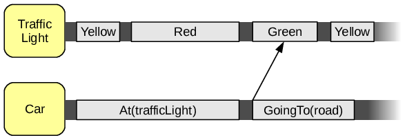
The figure above shows an example of synchronization; in the picture there are two state variables, TrafficLight and Car, both with their flexible timelines: tokens are allocated on them but they are free to move to a certain degree (the darker areas in the drawing) because of uncertainty. Let’s assume for now that the TrafficLight state variable is out of planner control, and that the planner must decide when the car can cross the traffic light to reach the road. Here, the GoingTo(x) value is the trigger of the synchronization, which is represented for simplicity by an arrow ending in Green, even if it is probably more complicated than just a constraint on the color of the traffic light. For example, it might be specified as follows:

The trigger is GoingTo(x)
x = road (that is, this set of rules does not apply if we are going somewhere else)
the trigger must come AFTER At(trafficLight)
the trigger must START AFTER the traffic light is Green
the trigger must START BEFORE the traffic light ceases to be Green

In this example, there are logical constraints on the value of parameters (2,3), temporal relations between the trigger and tokens on other timelines (4,5) and even on the same timeline (3).

Temporal Relations

Temporal relations are a key element of synchronization rules, because they allow to express temporal constraints between state variable values allocated on the same or different timelines.

More generally, temporal relations can be:

between two temporal intervals
between a temporal interval and a time point
between two time points

As [COU2016] points out, temporal relations between two intervals can be expressed by the means of four primitive relations between their start and end points:

A start-before-start_[lb,ub] B
A end-before-end_[lb,ub] B
A start-before-end_[lb,ub] B
A end-before-start_[lb,ub] B

where A and B are intervals, and [lb,ub] is another interval that specifies the distance between the two points considered.

Similarly, all temporal relations between an interval and a time point can be defined by combining the following primitives:

A starts-before_[lb,ub] t
A starts-after_[lb,ub] t
A ends-before_[lb,ub] t
A ends-after_[lb,ub] t

where A is an interval and t a time point, and [lb,ub] has the same meaning of the previous case.

Allen’s Relations

Some popular operators, vastly used in timeline-based planning, are Allen’s Relations. These are a set of 13 different operators that express all possible relationships between two time intervals, as shown in the following figure.

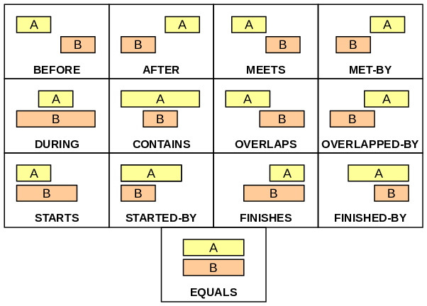
In timeline-based planning, these relations are usually extended to take some interval parameters to specify the amounts by which a relation holds. For example, the BEFORE relation uses a parameter to describe the distance between A’s end and B’s start; one parameter is also used by AFTER, STARTS, FINISHES and their opposites. Two parameters are used for the distances between the two start points and the two end points, respectively, by DURING, CONTAINS, OVERLAPS, OVERLAPPED-BY. Finally, MEETS, MET-BY and EQUALS don’t take parameters.

Controllability

As it was mentioned in section The Planner, not all the objects that are modeled in a domain file represent entities under the complete control of the planner; this is an important feature to have as it permits to describe also the environment, hostile conditions or adversaries, and in general external factors whose behavior cannot be determined by the planner, but can only be observed.

When reasoning about controllability, it is possible to distinguish among different levels: state variables can in fact be classified into completely uncontrollable, partially controllable and controllable.

External: state variables are components whose behavior is completely outside the control of the planner; the latter can only assume that the duration of each token remains inside the specified duration bounds, but it must assume that every schedule obeying to transition constraints and synchronization rules may be possible.
Partially Controllable: state variables are “normal” planned variables that the planner is generally able to control. These variables though have some values whose duration cannot be decided by the planner, and are hence called uncontrollable values; what this means is that the planner can decide when a state variable must assume an uncontrollable value, but it cannot decide when this value must be changed again: for these values, the state variable is treated by the planner as an external one. An important consequence is that the planner is forced to use flexible intervals for uncontrollable values, and this implies that all subsequent scheduled tokens on the same timeline, even if controllable, must be allocated using flexible intervals.
Controllable: state variables, also known as planned, are variables completely under the control of the planner, that can then decide when to trigger each transition.

In the example synchronization figure before, the TrafficLight variable is considered external: the planner’s duty is to control the car, and it cannot intervene to make the traffic light change its color as needed; what it can know, however, are the transition constraints (and possibly synchronization rules) that govern the traffic light behavior: so, for example, it knows which is the expected sequence of colors, and what the maximum durations associated to each light are, and it can use this knowledge when building a plan to govern the car’s behavior.

Resources

State variables (see section State Variables) are a very useful construct to model objects whose state can be expressed as symbolic, discrete values, and the examples given so far in this guide were appropriate to be expressed by state variables; sometimes however it is necessary to model entities having a numeric, “quantitative” state rather than a symbolic one.

Resources are this kind of construct; as state variables, they are components, and thus have timelines and tokens, but they are characterized by an amount which represents the quantity of resource that can be used.

Resources can be divided in two kinds: renewable and consumable.

Renewable Resources: are used to model objects who can yield a certain amount of the resource they represent (up to their capacity) for some time, and automatically claim it back when usage terminates. They can used to model occupation constraints, where some amount of space is used (provided it doesn’t exceed the capacity), but it is obviously automatically freed when resource utilization ceases.
Consumable Resources: instead don’t regain the lost amounts automatically, and must be explicitly “recharged” to be used again; they can be employed to model objects such as fuel tanks or batteries that can be used until they discharge, but that need to be refilled afterwards. Consumable resources are characterized by a minimum and a maximum value, representing the minimum amount of resource they can hold and their maximum capacity, respectively.

While state variables’ tokens represent a value that the state variable assumes for a certain amount of time, resources’ tokens are the actions that change their amount.

Renewable resources have only a possible action, the requirement of some amount of resource, represented as requirement(x), where x is the specified amount; when the token that represents this action terminates, the used amount is automatically returned.
Consumable resources have two possible actions, the consumption and the production of amounts of resource, which are written as consumption(x) and production(x) in analogy to the requirement action of renewable resources.

Resource actions can be used in synchronization rules in the same way of state variable values: as triggers in synchronizations, and as tokens involved in temporal relations.

For example, consider the case of a car which can advance for 20 km while consuming 1 liter of fuel; the car is modeled with a state variable, having among its values Advance(x), where x is the distance traveled, in meters; the car’s fuel tank is modeled as a consumable resource where its amount is expressed in milliliters; a synchronization might be written on Advance(x) containing a constraint EQUALS fuelTank.consumption(x/20). This constraint’s purpose is twofold: for one, it expresses the precondition for the tank to contain at least x/20 milliliters of fuel for the car to be able to advance; and, it makes the fuel tank actually decrease its amount if the car really advances. Note the usage of the EQUALS temporal relation, to mean that the token representing the consumption of fuel starts and ends at the same moments in which the token representing the advancing of the car do: in other words, that advancement and consumption happen simultaneously.

The DDL Language

The concepts explained in this guide need to be expressed in a planning language. The language that KeeN targets is called “DDL.3”: a detailed explanation of the language is outside of the scopes of this guide: the reader should be able to understand the examples in the KeeN User Guide, and to use KeeN, by just having a general understanding of Timeline-based planning, as explained here. If needed, a reference of the DDL language in EBNF form can be found here.

[1] To be precise we should say that a timeline describes the temporal evolution of a component, thus including resources too ↩.